Glomerulus Segmentation

Training an Unet++ with fastai to segment glomeruli.

Model Training Notebook

Here we train a Unet++ architecture with a pretrained efficientnet-b4 backbone from the awesome segmentation_models_pytorch library. Data loading, transforming, the actual training and, finally, exporting the newly trained model, we use fastai.

Here’s a running example of the model trained with this notebook.

Goal

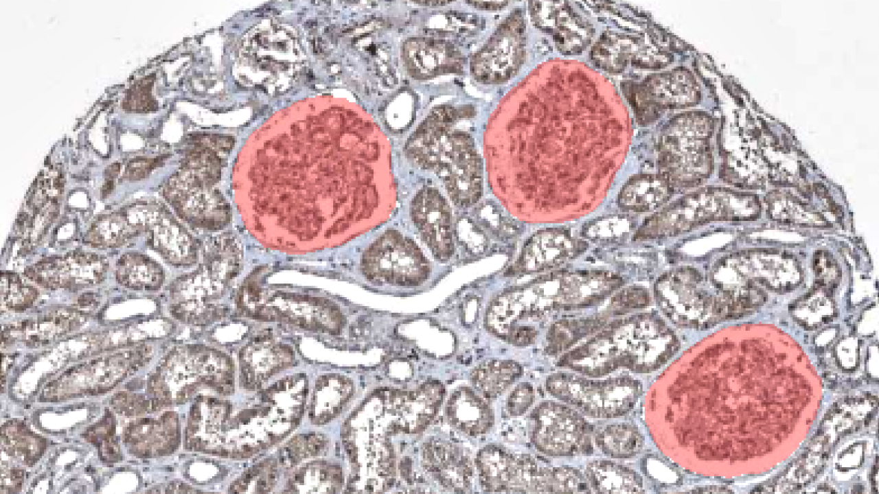
Segmenting glomeruli (an intricate structure in the kidney’s cortex in which the blood filtration happen), i.e. turning this

to this

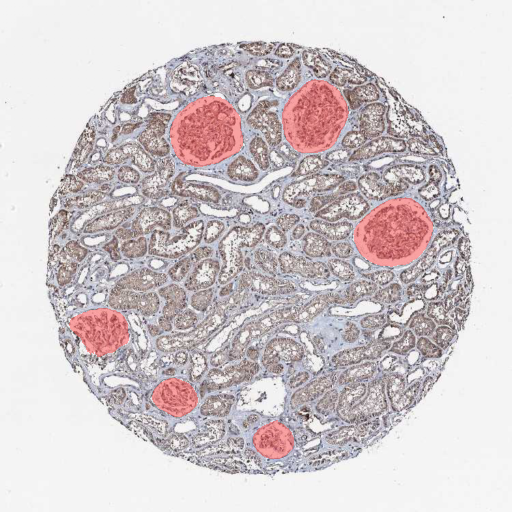
Data

I am using training data from the HuBMAP Challenge hosted on kaggle and a few dozen images downloaded from the Human Protein Atlas I annotated myself. (If you’re interested in how to do this, here a blogpost I wrote)

import numpy as np
import pandas as pd
import monai
from fastai.vision.all import *
import segmentation_models_pytorch as smp

ORGAN = "kidney"
TRAIN_BATCH_SIZE = 8 # Reduce this, if you run out of cuda memory
EFFECTIVE_BATCH_SIZE = 8 # This is the batch size that will be used for training
IMAGE_SIZE = 512
LR = 3e-4 
EPOCHS = 60
MODEL_NAME = f"smp_{IMAGE_SIZE}_{ORGAN}_added_data"
DATA_PATH = Path("../data/")

# Reproducibility
TESTSET_SEED = 93
TRAIN_VAL_SEED = 43

df = pd.read_csv(DATA_PATH/"train.csv") # This is the training set from the competition
fns = L([*get_image_files(DATA_PATH/"test_images"), *get_image_files(DATA_PATH/"train_images")]) # List of all competition images   
fn_col = [] # This will be a column in the dataframe, containing the filenames
for _, r in df.iterrows(): fn_col.append([fn for fn in fns if str(r["id"]) == fn.stem][0])
df["fnames"] = fn_col
df["is_organ"] = df.organ.apply(lambda o: o==ORGAN)
df = df[df.is_organ] # Only keep images with the organ we are interested in
assert df.organ.unique()[0] == ORGAN
df = df.drop(columns="organ data_source is_organ tissue_thickness pixel_size sex age".split()).copy()

# These are the images I added and that are annotated by me
add_images = get_image_files(DATA_PATH/"add_images/") 
add_images_masks = get_image_files(DATA_PATH/"segs/")

# The masks have the same name as the images, but with "_mask" appended
masks = [p.name[:-9]+".png" for p in add_images_masks] 

# Delete images without masks
images_to_delete = [p for p in add_images if p.name not in masks] 
for p in images_to_delete: p.unlink()

# This will contain the masks in the same order as the images
sorted_masks = [] 
for i in add_images:
    sorted_masks.append([p for p in add_images_masks if i.stem == p.stem[:-5]][0])

# Combine the competition data with the added data
add_df = pd.DataFrame({
    "fnames": add_images,
    "segmentation": sorted_masks,
    "is_add": [True]*len(add_images)
})
df["is_add"] = df.id.apply(lambda p: False)
combined_df = pd.concat([df, add_df])

# Setting aside a random testset
cut = int(0.1 * len(combined_df))
ind = np.arange(len(combined_df))
np.random.seed(TESTSET_SEED) # Always create the same testset
np.random.shuffle(ind)
test_ind = ind[:cut]
train_valid_ind = ind[cut:]
test_df = combined_df.iloc[test_ind,:].copy()
train_df = combined_df.iloc[train_valid_ind,:].copy()

The masks of the competition data are in run-length encoding, that’s why we need the following function. It converts the run-length encoding to a numpy array which we can use for training.

# From: https://www.kaggle.com/code/paulorzp/run-length-encode-and-decode/script
def rle_decode(mask_rle, shape):
    '''
    mask_rle: run-length as string formated (start length)
    shape: (height,width) of array to return 
    Returns numpy array, 1 - mask, 0 - background
    '''
    s = mask_rle.split()
    starts, lengths = [np.asarray(x, dtype=int) for x in (s[0:][::2], s[1:][::2])]
    starts -= 1
    ends = starts + lengths
    img = np.zeros(shape[0]*shape[1], dtype=np.uint8)
    for lo, hi in zip(starts, ends):
        img[lo:hi] = 1
    return np.reshape(img, shape)

CODES = ["Background", "FTU"] # FTU = functional tissue unit

def x_getter(r): return r["fnames"]
def y_getter(r): 
    # My additional annotations are saved as pngs, so I need to differ between the two
    if r["is_add"]: 
        im = np.array(load_image(r["segmentation"]), dtype=np.uint8)
        im = (im.mean(axis=-1) < 125).astype(np.uint8)
        return im
    rle = r["rle"]
    shape = (int(r["img_height"]), int(r["img_width"]))
    return rle_decode(rle, shape).T

btfms = aug_transforms(
    mult=1.2,
    do_flip=True,
    flip_vert=True,
    max_rotate=45.0,
    min_zoom=1.,
    max_zoom=1.5,
    max_lighting=0.3,
    max_warp=0.3,
    size=(IMAGE_SIZE, IMAGE_SIZE),
    p_affine=0.5
) # Data augmentation
dblock = DataBlock(blocks=(ImageBlock, MaskBlock(CODES)),
                   get_x=x_getter,
                   get_y=y_getter,
                   splitter=RandomSplitter(seed=TRAIN_VAL_SEED),
                   item_tfms=[Resize((IMAGE_SIZE, IMAGE_SIZE))],
                   batch_tfms=btfms)
dls = dblock.dataloaders(train_df, Path(".."), bs=TRAIN_BATCH_SIZE)

dls.train.show_batch()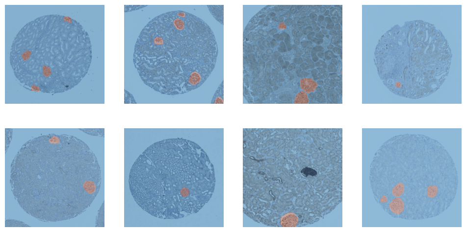

dls.valid.show_batch()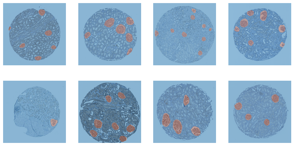

cbs = [
    GradientAccumulation(EFFECTIVE_BATCH_SIZE),
    SaveModelCallback(fname=MODEL_NAME),
]

model = smp.UnetPlusPlus(
    encoder_name="efficientnet-b4",        
    encoder_weights="imagenet",     
    in_channels=3,                  
    classes=2,                      
)

# Splitting model's into 2 groups to use fastai's differential learning rates
def splitter(model): 
    enc_params = L(model.encoder.parameters())
    dec_params = L(model.decoder.parameters())
    sg_params = L(model.segmentation_head.parameters())
    untrained_params = L([*dec_params, *sg_params])
    return L([enc_params, untrained_params])

learn = Learner(
    dls, 
    model, 
    cbs=cbs,
    splitter=splitter,
    metrics=[Dice(), JaccardCoeff(), RocAucBinary()])

learn.fit_flat_cos(EPOCHS, LR)

epoch	train_loss	valid_loss	dice	jaccard_coeff	roc_auc_score	time
0	0.727570	0.603148	0.085859	0.044855	0.322773	00:12
1	0.604307	0.516570	0.096767	0.050843	0.427407	00:11
2	0.508117	0.379248	0.522587	0.353718	0.314975	00:11
3	0.424914	0.302621	0.584612	0.413040	0.085511	00:11
4	0.353784	0.207627	0.712757	0.553709	0.128719	00:11
5	0.296790	0.142182	0.830598	0.710276	0.556589	00:11
6	0.250124	0.107157	0.849849	0.738903	0.781829	00:11
7	0.211806	0.088498	0.857634	0.750752	0.867223	00:11
8	0.180824	0.070990	0.859145	0.753071	0.888895	00:11
9	0.154632	0.061644	0.856697	0.749318	0.929199	00:11
10	0.133044	0.052796	0.868353	0.767336	0.953055	00:11
11	0.115005	0.046287	0.871848	0.772811	0.964127	00:11
12	0.099967	0.040762	0.883804	0.791800	0.971401	00:11
13	0.087097	0.037157	0.889235	0.800560	0.976527	00:11
14	0.076725	0.033152	0.899692	0.817673	0.979948	00:12
15	0.068125	0.031111	0.902548	0.822404	0.982294	00:11
16	0.060929	0.027760	0.910408	0.835549	0.984009	00:11
17	0.054637	0.027974	0.894529	0.809184	0.983233	00:11
18	0.049165	0.024334	0.911780	0.837864	0.986022	00:11
19	0.044277	0.024281	0.905008	0.826498	0.983716	00:11
20	0.040233	0.022132	0.913338	0.840498	0.986142	00:11
21	0.036737	0.021514	0.913032	0.839981	0.982759	00:12
22	0.033632	0.020441	0.919236	0.850543	0.988929	00:11
23	0.031428	0.021564	0.900877	0.819632	0.976978	00:11
24	0.029265	0.018416	0.922131	0.855513	0.990599	00:11
25	0.027243	0.017509	0.924026	0.858781	0.990082	00:11
26	0.025496	0.018210	0.916627	0.846087	0.983598	00:11
27	0.024097	0.017901	0.917531	0.847628	0.987033	00:11
28	0.022979	0.016894	0.920493	0.852697	0.986602	00:11
29	0.021918	0.018380	0.916335	0.845588	0.989573	00:11
30	0.020899	0.016375	0.920465	0.852650	0.988758	00:11
31	0.019700	0.014662	0.929562	0.868394	0.988694	00:11
32	0.018992	0.018643	0.906843	0.829563	0.989722	00:11
33	0.018747	0.016715	0.918087	0.848578	0.986600	00:11
34	0.018041	0.015872	0.918797	0.849792	0.982712	00:11
35	0.017152	0.015625	0.922364	0.855914	0.979253	00:11
36	0.016359	0.014718	0.925542	0.861403	0.977279	00:11
37	0.015855	0.012931	0.932580	0.873676	0.987032	00:11
38	0.015509	0.012442	0.932764	0.873999	0.990109	00:11
39	0.015077	0.011627	0.936922	0.881329	0.989619	00:11
40	0.014742	0.011964	0.934999	0.877933	0.987285	00:11
41	0.014460	0.011784	0.937937	0.883128	0.990435	00:11
42	0.014327	0.013164	0.928118	0.865877	0.985723	00:11
43	0.014337	0.012003	0.934332	0.876757	0.987117	00:11
44	0.014002	0.012138	0.935304	0.878470	0.988768	00:11
45	0.013552	0.011391	0.936339	0.880298	0.987371	00:11
46	0.013122	0.012408	0.929143	0.867663	0.983431	00:11
47	0.012708	0.011765	0.932473	0.873489	0.990839	00:12
48	0.012281	0.010892	0.938805	0.884668	0.987427	00:11
49	0.011792	0.010427	0.941303	0.889115	0.986761	00:11
50	0.011579	0.011140	0.938671	0.884429	0.982990	00:11
51	0.011452	0.010431	0.945001	0.895737	0.985848	00:11
52	0.011334	0.010210	0.943139	0.892396	0.987449	00:11
53	0.011300	0.011088	0.937227	0.881870	0.987982	00:11
54	0.011329	0.010670	0.937806	0.882895	0.988177	00:11
55	0.011342	0.010610	0.937321	0.882035	0.989792	00:11
56	0.011146	0.010468	0.938884	0.884808	0.988132	00:11
57	0.011024	0.010291	0.940346	0.887408	0.988785	00:11
58	0.010618	0.010369	0.939683	0.886228	0.988485	00:11
59	0.010563	0.010375	0.939610	0.886099	0.988654	00:11

Better model found at epoch 0 with valid_loss value: 0.6031481027603149.
Better model found at epoch 1 with valid_loss value: 0.516569972038269.
Better model found at epoch 2 with valid_loss value: 0.3792479634284973.
Better model found at epoch 3 with valid_loss value: 0.302621066570282.
Better model found at epoch 4 with valid_loss value: 0.20762743055820465.
Better model found at epoch 5 with valid_loss value: 0.14218230545520782.
Better model found at epoch 6 with valid_loss value: 0.10715709626674652.
Better model found at epoch 7 with valid_loss value: 0.0884983241558075.
Better model found at epoch 8 with valid_loss value: 0.07099024951457977.
Better model found at epoch 9 with valid_loss value: 0.06164400279521942.
Better model found at epoch 10 with valid_loss value: 0.0527963824570179.
Better model found at epoch 11 with valid_loss value: 0.046286918222904205.
Better model found at epoch 12 with valid_loss value: 0.04076218977570534.
Better model found at epoch 13 with valid_loss value: 0.037156544625759125.
Better model found at epoch 14 with valid_loss value: 0.0331517718732357.
Better model found at epoch 15 with valid_loss value: 0.031111164018511772.
Better model found at epoch 16 with valid_loss value: 0.027760174125432968.
Better model found at epoch 18 with valid_loss value: 0.024333978071808815.
Better model found at epoch 19 with valid_loss value: 0.024281086400151253.
Better model found at epoch 20 with valid_loss value: 0.022132011130452156.
Better model found at epoch 21 with valid_loss value: 0.021513625979423523.
Better model found at epoch 22 with valid_loss value: 0.020441483706235886.
Better model found at epoch 24 with valid_loss value: 0.018416451290249825.
Better model found at epoch 25 with valid_loss value: 0.017508765682578087.
Better model found at epoch 28 with valid_loss value: 0.016893696039915085.
Better model found at epoch 30 with valid_loss value: 0.016375476494431496.
Better model found at epoch 31 with valid_loss value: 0.0146623644977808.
Better model found at epoch 37 with valid_loss value: 0.012930507771670818.
Better model found at epoch 38 with valid_loss value: 0.01244184747338295.
Better model found at epoch 39 with valid_loss value: 0.01162666454911232.
Better model found at epoch 45 with valid_loss value: 0.011391145177185535.
Better model found at epoch 48 with valid_loss value: 0.010892268270254135.
Better model found at epoch 49 with valid_loss value: 0.010426941327750683.
Better model found at epoch 52 with valid_loss value: 0.010209585539996624.

learn.load(MODEL_NAME)

Saved filed doesn't contain an optimizer state.

<fastai.learner.Learner at 0x7f2dd019eac0>

learn.show_results()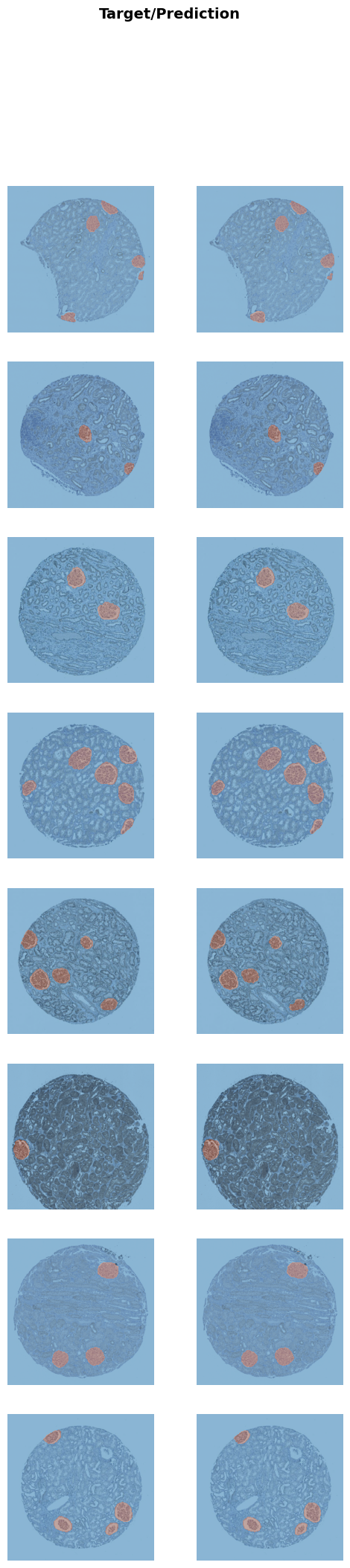

# Create a dataloader from the testset
test_dl = dls.test_dl(test_df, with_labels=True)
dice_func = monai.metrics.DiceMetric(include_background=False, reduction="mean")

# This function steps through the different thresholds and returns the best one
def get_best_threshold(learn, dl, metric_func, n_steps=17):
    """
    Tests `n_steps` different thresholds.
    Return the best threshold and the corresonding score.
    """
    thresholds = torch.linspace(0.1, 0.9, n_steps)
    results = []

    res = learn.get_preds(dl=dl, with_input=False, with_targs=True, act=partial(F.softmax, dim=1))
    
    for t in thresholds:
        metric_func((res[0][:,1]>t).unsqueeze(1), res[-1].unsqueeze(1))
        metric = metric_func.aggregate().item()
        metric_func.reset()
        results.append((round(t.detach().cpu().item(), ndigits=3), metric))

    return sorted(results, key=lambda tpl: tpl[1], reverse=True)[0]

best_threshold, _ = get_best_threshold(learn, dls.valid, dice_func)
best_threshold

0.6

And now we test the model on the training, validation and test set with the best threshold.

def test_model(learn, dl, metric_func, threshold=0.5):
    res = learn.get_preds(dl=dl, with_input=False, with_targs=True, act=partial(F.softmax, dim=1))
    metric_func((res[0][:,1]>threshold).unsqueeze(1), res[-1].unsqueeze(1))
    metric = metric_func.aggregate().item()
    metric_func.reset()
    return metric
    
train_dice = test_model(learn, dls.train, dice_func, threshold=best_threshold)
valid_dice = test_model(learn, dls.valid, dice_func, threshold=best_threshold)
test_dice  = test_model(learn, test_dl,   dice_func, threshold=best_threshold)

for s, d in zip(("Training Dice:", "Valid Dice", "Test Dice"), (train_dice, valid_dice, test_dice)):
    print(s, d)

Training Dice: 0.9252251982688904
Valid Dice 0.9271063208580017
Test Dice 0.9414731860160828

# Save and export the model
BEST_MODEL_NAME = f"unetpp_b4_th{int(best_threshold*100)}_d{str(test_dice)[2:6]}"
learn.save(BEST_MODEL_NAME)
learn.export(BEST_MODEL_NAME+".pkl")

A live version of this model is deployed on a huggingface space.